Facts about Facts: Organizing Fact Tables in Data Warehouse Systems

The process of defining your data warehousing system (DWH) has started. You’ve outlined the relevant dimension tables, which tie to the business requirements. These tables define what we weigh, observe and scale. Now we need to define how we measure.

Fact tables are where we store these measurements. They hold business data that can be aggregated across dimension combinations. But the fact is that fact tables are not so easily described – they have flavors of their own. In this article, we’ll answer some basic questions about fact tables, and examine the pros and cons of each type.

What Are Fact Tables?

In the most general sense, fact tables are the measurements of a business process. They hold mostly numeric data and correspond to an event rather than a particular report.

The most important feature of a fact table, besides measures, is grain. Grain defines what level of detail is observed for a particular event. (Compare this with the phrase ‘fine-grain controls’, which means that users can control very small details for their account.)

The more detailed the fact table’s grain, the better it will handle unpredictable business requirements. The downside of greater grain is that more physical space is required for data storage. It can also cause slower performance.

How Are Fact Tables Structured?

A general fact table consists of two main attribute groups:

• Foreign keys to dimensional tables
• Measures

Foreign keys are self-explanatory; degenerate dimensions also belong to this group. A degenerate dimension is a dimension key with no parent dimension table. They occur when all the important information about the dimension is already in the fact table. Examples include various control header numbers, ticket numbers, order numbers, etc.

Measures (i.e. metrics or business facts) in a fact table can be:

• Additive: summable across any dimension
• Semi-additive: summable across some dimensions
• Non-additive: not summable (e.g. various ratios)

Besides measures and foreign keys, there can be many technical columns. Technical columns are useful for auditing and low-level maintenance of the model. Timestamps, which are used to mark when insertions or updates occur in the fact table, are a common example of a technical column.

To illustrate a generic fact table, let’s look at a very simple star schema:

In this model, we have a single fact table surrounded by three dimension tables. Our foreign keys for the fact table include:

• time_id – refers to the time dimension table (dim_time)
• product_id – refers to the product dimension table (dim_product)
• store_id – refers to the store dimension table (dim_store)
• pos_transaction – a degenerate dimension. This is all the information about POS we need, so we can store it here. There’s no reason to build another dimension table.

Our measure key group consists of:

• sales_quantity – The sales of one product at one time in one store. This measure is additive.
• sales_price – The price of an item as sold in the store. This is a non-additive measure.

There is one technical column, time_inserted, that stores the time when a row is inserted.

Now that we have a general idea of fact tables, we’ll dig into their different flavors. There are four types of fact tables: transaction, periodic snapshot, accumulating snapshot and factless fact tables.

Every flavor serves a purpose in representing the underlying business which the data warehousing system supports. However, before we delve into what these different fact tables do, let’s talk about an important common factor: sparsity, or the proportional amount of data stored in a fact table. Sparsity is related to grain, and it has an effect on query performance.

What Is Fact Table Sparsity?

When designing a fact table, consider its sparsity – i.e. what number of the table’s rows are populated versus how many are empty. If we fill the fact tables from many underlying tables, it is wise to estimate sparsity. We make the estimation based on the level of grain in the fact table. If your fact table matches the underlying source table, you can use the cardinality of the underlying table to calculate sparsity.

To compute sparsity, first we find the fill ratio – that is, the number of non-empty cells to total cells. To figure the fill ratio, divide the number of rows in the source table by the number of distinct rows in each dimension table. Sparsity is then calculated as 1-(f), where f = fill ratio.

Example:

Suppose we fill the fact_retail_sale table from two sources: a database table with 100,000 rows and a spreadsheet with 20,000 rows. These rows are filled on a yearly basis. The dimension tables are: dates (365 rows), products (100 rows) and stores (1,000 rows).

We calculate sparsity as:

1-(100,000 + 20,000)/(365*100*1,000) = 0.99671

This fact table is sparse, because less than 1% of its rows have non-zero values.

A good rule of a thumb is that we consider anything under 2% very sparse; anything above that is not so sparse.

Transaction Fact Tables

This is the simplest and most common type of fact table. The grain of this type is one row per transaction, or one row per line on a transaction. The grain of a transaction fact table is a point in space and time. They hold the smallest of business details.

As a transaction happens, extensive context about it is captured. This context creates lots of detail in the dimension tables, so we expect a lot of them.

Once we insert a row in a transaction table it is rarely, if ever, revisited. This leads us to consider specific techniques for populating these types of tables. No updates means a much simpler ETL (extract, transform, and load process).

Pros: Higher granularity enables monitoring of detailed business activities.

Cons: Performance issues in query. Difficulty in interpreting trend behaviors at fixed points in time.

An Example of a Transaction Fact Table

Let’s look at a typical financial star schema:

We record every single account action in the fact table. Sample data from this table includes:

Note: time_date is represented as it is shown in the dim_time dimension, and the technical column is ignored.

As the account owner completes transactions, such as depositing and withdrawing money, we record every action.

With this structure we can answer questions like: How many transactions per day does our business process? What is the average amount withdrawn in one day? etc.

Periodic Snapshot Fact Tables

Periodic snapshot tables record the cumulative performance of the business at predefined periods of time. A predetermined interval for taking snapshots is the key: daily, weekly, monthly, etc. The results are saved in the periodic snapshot fact table.

This type of fact table gives us a lot of leeway: we can incorporate any information that describes activity over a time period.

Moving from a transaction to a periodic table is possible. (There are some neat algorithms in SQL that deal with this, as we will see in upcoming articles.) It is only a matter of adding up the transactions from one snapshot to another. Just as transaction fact tables have many dimensions, the snapshot usually has fewer dimensions.

Pros: Performance gain, longitudinal view of business, physical compactness.

Cons: Lower grain.

An Example of a Periodic Snapshot Fact Table

Let’s consider another financial star schema:

Let’s assume that we built this fact table and its data mart from the same source as the previous example. We could have even built this fact table from the data in the previous fact table.

We need to show the balance_amount on every snapshot date; in this case, the snapshot granularity is one day. We aggregate all outbound transactions on a daily basis, and the deposit type is adding and withdrawal is subtracting. The result is:

Note: We present time_date as it is shown in the dim_time dimension and the technical column is ignored.

Now we can answer some common business questions, like: How many days does a customer carry a positive account balance in one month? What is the average balance of a specific type of customer each month? etc.

Reorganizing a Periodic Snapshot Fact Table

You may have noticed some redundancy in the data displayed in the previous example. Sometimes even the snapshot fact table is too big and performance takes a tumble. What to do then? We can reorganize our snapshot fact table into something more compact.

We’ve added two new columns, date_from and date_to. They represent the period of time in which the balance_amount was valid.

The data in this table would look like this:

Every time the balance_amount changes, we close the time period and open a new one.

Notice that the date_to column contains a non-inclusive time delimiter. We have to take this into account when we query data. We also find one interesting date – 31/12/9999. This date demonstrates that the last row is the last known balance. We will update it when the balance changes.

Below, we can see the SQL we use to query a snapshot at a particular date (:date).

SELECT ft.*
FROM
	fact_account_snapshot ft
WHERE date_from <= :date
	     and :date < date_to

Accumulating Snapshot Fact Tables

The accumulating snapshot fact table is the least common type, but it’s also by far the most interesting and challenging. We use this table type when we represent processes that have a definite beginning and end.They are most appropriate when users must perform pipeline and workflow analysis.

Accumulating snapshot tables usually have multiple date foreign keys, each corresponding to a major milestone in the workflow. And while the processes captured in this type of table have beginnings and ends, intermediate steps are recorded as well.

Transaction fact tables may have several dates associated with each row; the accumulating fact table allows for many of the date values to be unknown when the row is first loaded. This is unique among fact tables, and it can lead to anomalies – incomplete dimensions – in dimensional modeling.

We solve this by adding a default value to the missing fields in the fact table and the appropriate dimension table. As we revisit the row containing specific workflows, we must implement a different type of ETL for working with these tables.

Pros: Enables complex analysis of tables and workflow analysis.

Cons: High ETL complexity.

An Example of an Accumulating Snapshot Fact Table

In this example, imagine that we have to analyze the effectiveness of our loan approval process, from initial application to final funding. Obviously, we first need to prepare our data!

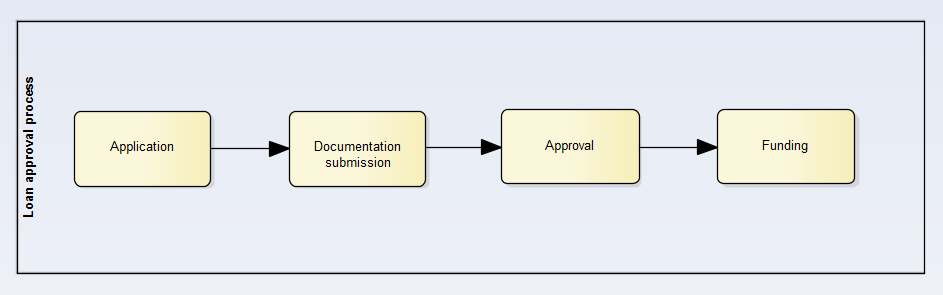
Our loan approval process has four steps:

1. Loan application from a bank customer
2. Submission of complete documentation needed for loan approval (appraisal, credit status etc.)
3. Approval of the loan application from a higher-ranking bank employee
4. Funding the loan

One row in our fact table represents one instance of this process.

As we see in the data table, not all our workflows are complete; future actions will make us revisit the fact table and update our data. This is the main difference between this and other types of fact table.

Some questions that we can answer with this type of fact table are: Where is the bottleneck in the loan approval process? What is causing it? What is the average time needed for end-to-end approval? etc.

Let’s look at the data from the fact table. We’ll split the display into two tables:

Looking at the data, we see a strange date: 01.01.1900. This date represents a missing or “not yet filled” date. It is more practical to have a default value for missing key data so we don’t have abnormalities when we do a roll-up.

We can also draw some conclusions from this data. Bigger loans take more time to process. This is normal because they need more documentation and safety checks. Smaller loans complete the process much faster.

Factless Fact Tables

This inconspicuous fact table can also be found in the data warehouse modeling world. The factless fact table does not have any measurements; it only holds foreign keys to dimensional tables. This information is enough to answer relevant business questions.

Pros: Simplicity

Cons: Limited usefulness

An Example of a Factless Fact Table

In the following example, we see a star schema featuring a factless fact table. The schema is used for tracking student attendance, with four dimensional tables representing courses, facilities, dates, and departments.

With this schema, we can find answers to questions like: How many students attended a class last month? What course has the lowest attendance this year? What facility is not being used? etc.

A simple query can answer the last question. The code would be:

SELECT course_id, count(*) number of attendance
FROM
	fact_student_attendance ft
	JOIN dim_course dc ON (dc.course_id = ft.course_id)
	JOIN dim_time dt ON (dt.time_id = ft.time_id)
WHERE dt.time_year = 2016
GROUP BY course_id
ORDER BY count(*) desc

Our answer is returned in the first line of the query.

Fact tables are the meat of the data warehousing world. Their size can equal many terabytes, and they take the most space in a data warehouse. An error early in the fact table design process generates many problems, which don’t get easier to solve as the warehouse evolves!

It is possible to reorganize data from one type of fact table to another. We will explore techniques to do this in an upcoming post. What about your experiences with different types of fact tables? Did you manage to mix them in some new and exciting way? If you did, let me know.