Improve Your Financial Reporting With Data Warehousing

Financial institutions, especially banks, usually have really large datasets. To use that data, it must be stored in such a way that it is easily available for generating reports. The trend now is to use a data warehouse to store all your relevant data, and to use smaller data marts (subsets of the warehouse) to keep specific data sets in a convenient place.

But where to start? In this article, we’ll look at one possible solution, similar to a project I worked on in the past. While we implemented a different approach, the underlying idea was very similar.

Data needs to be grouped based on an institution’s desired reporting categories. These categories play the role of dimension tables in our model, while the fact table is used to store the financial data we want to present. The fact table and the dimension tables form the reporting data mart.

The Problem with Financial Reporting

Reporting is crucial to tracking performance and making sound business decisions. There are also many reports required by regulators. As you might imagine, creating these different kinds of reports presents some challenges.

Here’s another issue: the EU (and other national and international bodies) has its methodology and national central banks have their methodologies. If a bank belongs to an international group, with headquarters located in a different country, it will probably need to create additional reports that use the internal group methodology.

Moreover – the worst of all, from a design perspective! – methodologies change over time. Most banks have been in business for many decades, and there is a lot of diversity in the applications and technologies used. Add changing regulations to that and it becomes messy.

Usually banks will use one core application with modules for specific purposes (e.g. credit application, call center application, etc.) Most reporting can’t be done unless data is aggregated at a single location. We could encounter many different problems during this integration/aggregation phase. For example, there could be different IDs for the same client, record errors, or incomplete data.

Data Warehouses and Marts: The Source of the Solution

In this article, we’ll discuss building a reporting data mart as a solution to difficult data aggregation. We’ll transform data and migrate it from external systems to a data warehouse, which will store this information.

The main advantage is that the data warehouse structure will stay the same regardless of changes to operational applications or regulations. This way, anyone who has to generate reports will be able to use predefined queries and report templates. Fractional CFO consulting services can use this strong data architecture to improve financial decision-making, optimize resource allocation, and forecast better to manage financial risks and opportunities. They’ll spend less time dealing with technicalities and have more time to use their expertise to interpret results.

First, we’ll take a look at the data model. Next, we’ll briefly describe how to import data into our warehouse and how to create a few simple reports out of it.

A Quick Introduction to the Model

The main dilemma is how to organize our data: snowflake schema or star schema. In addition, we need to define dimensions and granulation. And we should also plan for future needs.

First of all, we’ll stay realistic. We won’t include all possible dimensions, but we’ll add the ones currently needed and any that could be required in the relatively near future.

Our model is basically a star schema; it has one fact table, seven dimension tables, and one dictionary table.

In the fact table, only three values will represent financial data; the dimension tables will represent categories we want to use in reporting. The dim_city table is used twice, while the region table is a dictionary used to relate cities with their regions.

Let’s look at these tables in detail before we move on to transforming the data.

The Fact Table

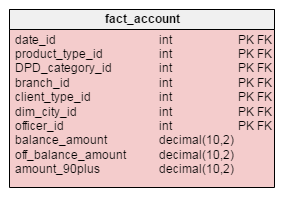
Our model has only one fact table: the fact_account table. This table stores three values we want to use in our reports:

• balance_amount – the sum of the on balance amount
• off_balance_amount – the sum of the off balance amount
• amount_90plus – the sum of the on balance and off balance amounts, but only amounts that are 90 or more days past due (DPD). So, suppose an account holder has €500 with DPD=93, €600 with DPD=63, €600 with DPD=33 and €600 with DPD=3. We’ll take only the first amount, €500, into this sum because it is more than 90 days past due.)

The other seven attributes are references to the dimension tables. Together, they form the primary key of the fact table.

The organization here is almost the same as the one presented in this article.

Dimensions

The dimensions used in our model are the ones most commonly used in reporting. There are many others that could be added, but these will serve our purpose.

Each dimension table uses its first column as an ID. This is an integer data type with its Auto_increment property set to “Yes”.

The second attribute in each dimension table is the alternate key. This will prevent anyone adding the same value more than once. We could use these values to map IDs from operational systems to our internal IDs.

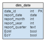
The most important dimension for reporting is the time dimension. Every record from the fact table will have a date assigned in the dim_date table. We’ll use the following attributes to describe the time dimension:

• report_date – the actual report date
• report_month – is the month’s ordinal number (e.g. 1 = January, 2 = February)
• report_year – the report year (2016, 2017)
• report_quarter – the report quarter (2016/Q1, 2016/Q2)
• EoM – the last date in month report_date belongs to (e.g. for report date 15.6.2016, EoM is 30.6.2016)
• EoY – the last date in year report_date belongs to (e.g. for report date 15.6.2016, EoY is 31.12.2016)

This way we’ll store records granulated on a daily level, but we’ll also have fast access to monthly, quarterly and yearly statistics. Of course, using five additional attributes (report_month, report_year, report_quarter, EoM and EoY) is redundant, but we’ll go with it because it will simplify future queries by quite a lot. On the other hand, we won’t lose significant memory. In one year, we’ll have 365 new records in the dim_date table, so the redundancy will cost us 1,825 additional values (365 days * 5 records per day). We can live with that.

This is the only dimension table where new values will be added on a regular (daily) basis. All other dimension tables will primarily contain the same values; new values will be added only if we face business changes (e.g. opening a new branch or introducing a new product).

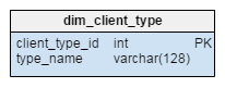
The purpose of the dim_client_type table is obvious by its name. Client segmentation is used because different client types have different behaviors. Some of the values we could expect in this dimension are “Private individual”, “SME/SMB” (small or medium-sized enterprise/business), or “Corporate”.

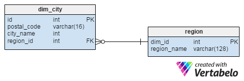
The dim_city dimension is a dictionary that holds a list of all the cities where we operate. The postal_code and the city_name attributes form the alternate key of the table. The city_name attribute holds the real name of the city, while region_id is a reference to the region dictionary table.

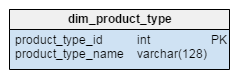
One of the more commonly used categories in financial reporting is the product type category. We’ll define this category by its name. Values we expect to encounter in this table are: “housing loan”, “mortgage loan”, “car loan”, or “current account”.

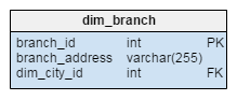
Most banks generate reports based on the branch where the account was opened.

The branch_address attribute stores this information and also plays the role of the alternate key. Each branch is related with the city where it’s located. Note: the city where the client operates and the city where the account was opened don’t have to be the same.

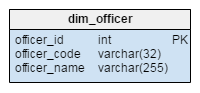
The dim_officer dimension stores data about all employees who can create an account. The officer_code attribute is the unique value and the alternate key of the table. An officer is not strictly related to a branch, so we can use both of them as separate dimensions.

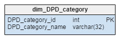
The days past due (DPD) dimension is very important in the analysis of loan performance. Usually, loans that are 90 or more DPD are treated as non-performing loans. Any loan in this category usually means that clients can’t fulfill their obligations on time. They’ll be offered restructuring or some other approach. Values expected in this table are: “0 days”, “1 to 30 days”, “31 to 60 days”, “61 to 90 days” etc. As you can see, the dim_DPD_category table stores these values.

There are many more dimension tables we could add to this. My first thought was to add another time dimension that would store when the account was created. It could be updated on a monthly basis. Accounts can change over time; ten years ago, maybe the conditions to get credit were much stricter than they are today, or perhaps terms were different. All this information could be useful, but for the purposes of illustration we will just limit ourselves to what we have.

The model is now defined and described. We could end the article here but I did promise to go into more detail about data transferal and aggregation. So let’s carry on. We’ll next consider adding new values in the dimension tables and importing aggregated data into the fact table. After that, we’ll see how to generate reports for end users.

Adding New Data to Dimension Tables

Before we add new values to the fact table, we have to check if there are any values we need to add to the dimension tables. We’ll check values that are used as alternate keys. If a new value doesn’t belong to the current set of values, we’ll add a new record in the dimension table.

We should expect to add at least one new value each day: a new date in the dim_date dimension table. Assuming that we have a list of new dates we want to add in the new_dates table, we should use a query like the one below to detect which dates we need:

SELECT

	new_dates.new_date AS new_report_date,
	MONTH(new_dates.new_date) AS new_report_month,
	YEAR(new_dates.new_date) AS new_report_year,

	CONCAT(YEAR(new_dates.new_date), "/",

	(CASE
		WHEN MONTH(new_dates.new_date) <= 3 THEN 'Q1'
		WHEN MONTH(new_dates.new_date) <= 6 THEN 'Q2'
		WHEN MONTH(new_dates.new_date) <= 9 THEN 'Q3'
		WHEN MONTH(new_dates.new_date) <= 12 THEN 'Q4'
	 	ELSE "Error"
	END)

	) AS new_report_quarter,

	IF (MONTH(new_dates.new_date) = MONTH(DATE_ADD(new_dates.new_date, INTERVAL 1 DAY)), False, True) AS new_EoM,
	IF (YEAR(new_dates.new_date) = YEAR(DATE_ADD(new_dates.new_date, INTERVAL 1 DAY)), False, True) AS new_EoY

FROM
	`new_dates`
	LEFT JOIN dim_date ON new_dates.new_date = dim_date.report_date

WHERE
	dim_date.report_date IS NULL

After adding new values in all dimension tables, we’re ready to add a new date into the fact table. Once again, we would use the alternate key to map to the appropriate primary key value.

Now that we’ve seen how to add data, let’s look at the final steps in our process: transforming the data into reports.

Creating New Reports and the ETL Process

In data analytics, the process of moving data from various applications to a data warehouse is known as ETL – extract, transform, and load.

With data inside our warehouse, we’ve already done the extracting. Now we’re ready to create some predefined queries that will return reports or extract the data needed to create more complex reports in other tools.

The main benefit of creating predefined queries or procedures is that end users won’t have to deal with any changes as they happen. The structure of our data mart will remain the same, and any changes in the actual ETL process will be handled by the IT team.

We can expect that a business user won’t need all the historical data. Most of the time, they’ll use data related to the current and the previous year. We could create a data mart that contains only the relevant data. This would improve performance and speed up the process since we would use notably smaller data sets.

We’ll take a look at a few predefined queries. The query below returns sum balance, off balance, and 90plus (90 DPD) amounts for:

• The last day of each month in 2016
• All housing loans
• Clients with regular payments and 0 DPDs

dim_date.report_date,
	SUM(fact_account.balance_amount) AS balance,
	SUM(fact_account.off_balance_amount) AS offbalance,
	SUM(fact_account.amount_90plus) AS '90plus'

FROM
	fact_account
	INNER JOIN dim_date ON fact_account.date_id = dim_date.date_id
	INNER JOIN dim_product_type ON fact_account.product_type_id = dim_product_type.product_type_id
	INNER JOIN dim_DPD_category ON fact_account.DPD_category_id = dim_DPD_category.DPD_category_id

WHERE
	dim_date.report_year = 2016
AND dim_date.EoM = True
	AND dim_product_type.product_type_id = "housing loan"
	AND dim_DPD_category.DPD_category_name = "0 days"
GROUP BY
dim_date.report_date

The query below returns the sum of balance, off-balance and 90plus amounts grouped by year and product type, but only for dates that are marked as the end of that year.

SELECT

	dim_date.report_year,
	dim_product_type.product_type_name,
	SUM(fact_account.balance_amount) AS balance,
	SUM(fact_account.off_balance_amount) AS offbalance,
	SUM(fact_account.amount_90plus) AS '90plus'

FROM
	fact_account
	INNER JOIN dim_date ON fact_account.date_id = dim_date.date_id
	INNER JOIN dim_product_type ON fact_account.product_type_id = dim_product_type.product_type_id

WHERE
	dim_date.EoY = True
GROUP BY
	dim_date.report_year,
	dim_product_type.product_type_name

Creating a data warehouse is not an easy process, especially in organizations that house large amounts of data and are obliged to create many different reports. Even the process of describing what is needed is very demanding.

Business experts, especially in the financial industry, expend too much effort trying to solve technical problems. This often means they lack the time to use their expertise where they primarily should. If you experience this problem, don’t hesitate to build yourself a data warehouse. It will be hard work, but once it’s completed you’ll enjoy the benefits.