Building an Information Mart With Your Data Vault

In the 3^rd post in this series, we looked at how we prepare data for use with a concept called the Business Data Vault. Now, in this final part, I will show you the basics of how we project the Business Vault and Raw DV tables into star schemas which form the basis for our Information Marts.

Raw Data Mart vs. Information Marts

As of Data Vault 2.0, the terminology changed a bit to be more precise. With DV 2.0 we now speak of “Information Marts” rather than just “Data Marts”.

Why?

Because truly when we build a star schema (or any style reporting table) on top of the DV, it usually involves some level of translation, transformation, or application of soft business rules (a la Business Vault). As such, our goal is to turn data into information that is useful for making business decisions.

On the other hand we also speak of what are best called Raw Data Marts. These are structures built on top of the Raw Data Vault by simply joining some of the DV tables together. The Raw Data Mart is an excellent option for agile data warehouse projects. I have used these on many occasions to get the raw, uncleansed, source data in front of the business users early on in a project. Confronted with the true (and often ugly) nature of their source data, I find that many business users find it much easier to then articulate the real business rules they need applied for the final reports (i.e., Information Marts).

In the next sections I will show you how to build Facts and Dimensions for both a Raw Mart and an Information Mart.

Dimensions

The simplest dimension is easily built by joining of a Hub and a Satellite. First you must decide if you need a Type 1 or a Type 2 dimension.

Type 1 Dimension for a Raw Data Mart

For a Type 1, which shows the most current values for all the attributes, we can use the Hub Key as the surrogate primary key (PK) for the dimension. I suggest using the existing Hub Key (the MD5 hash column) as it is already unique and will save you the processing of generating a typical integer surrogate for the dimension. This will save you processing time and allow you to load fact tables before or in parallel with the dimension. All the other columns in a Dimension will come from the contributing Hub and Satellite.

In the case of wanting to build a dimension for Countries, the following SQL can be used for a Type 1 Country Dimension:

SELECT
  HC.HUB_COUNTRY_KEY AS DIM1_COUNTRY_KEY,
  HC.COUNTRY_ABBRV,
  SC.COUNTRY_NAME,
  SC.SAT_Load_DTS AS EFFECTIVE_DTS,
  SC.SAT_Rec_SRC  AS REC_SRC
FROM
HUB_COUNTRY HC, SAT_COUNTRIES SC
WHERE HC.HUB_COUNTRY_KEY = SC.HUB_COUNTRY_KEY
 AND SC.SAT_Load_DTS =
       (
        SELECT
         MAX(S2.SAT_Load_DTS)
        FROM
         SAT_COUNTRIES S2
        WHERE
         HC.HUB_COUNTRY_KEY = S2.HUB_COUNTRY_KEY
       )

As you can see, I renamed the Hub Key to be DIM1_COUNTRY_KEY. DIM1 indicating this is a Type1 slowly changing dimension. For “as-of” date, I have aliased the Sat Load Date to be called EFFECTIVE_DTS. Then, to ensure we are only looking at the current values for every Country, I included a Max(Load Date) type subquery on the Load Date.

In Figure 1 you can see the Raw Vault model side-by-side with the projected Type 1 Dimension.

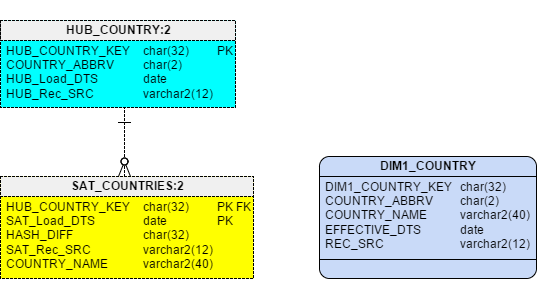
Figure 1 – Projecting a Type 1 Dimension from a Raw Vault

For implementation, you simply build the dimension table, then load it using the SQL code shown above.

Type 2 Dimension for a Raw Data Mart

Projecting a Type 2 slowly changing dimension (SCD) is only slightly more difficult. Since a Type 2 tracks changes to values over time (just like a Satellite), that means there may be more than one row in the Dimension for each business key (in this case COUNTRY_ABBRV). Because of that, you cannot use the Hub Key as the primary key on the Dimension.

If you are using DV 2.0, then I suggest you create the surrogate PK by using the same MD5 hash approach as we did in the Raw Vault. So to get a unique key in this case, you need to create a hash based on the Business Key plus the SAT_LOAD_DTS.

For Oracle the Hash looks like this:

dbms_obfuscation_toolkit.md5(upper(trim(HC.COUNTRY_ABBRV))  || '^'  ||
TO_CHAR(SC.SAT_Load_DTS, 'YYYY-MM-DD'))

The entire query to build a Type 2 SCD for Country looks like this:

SELECT
  dbms_obfuscation_toolkit.md5(upper(trim(HC.COUNTRY_ABBRV))
  || '^'
  || TO_CHAR(SC.SAT_Load_DTS, 'YYYY-MM-DD')) AS DIM2_COUNTRY_KEY,
  HC.COUNTRY_ABBRV,
  SC.COUNTRY_NAME,
  SC.SAT_Load_DTS AS EFFECTIVE_DTS,
  LEAD(SC.SAT_Load_DTS) 
       OVER (PARTITION BY SC.HUB_COUNTRY_KEY 
       ORDER BY  SC.SAT_Load_DTS) AS EXPIRE_DTS,
  SC.SAT_Rec_SRC AS REC_SRC
FROM
  HUB_COUNTRY HC,
  SAT_COUNTRIES SC
WHERE
  HC.HUB_COUNTRY_KEY = SC.HUB_COUNTRY_KEY

Since this is a Type2, in addition to wanting to see and effective date (like in the Type 1), most users also need either an Expiration Date or a Current Flag so they can easily report on current or historical values. In this example I chose to create an EXPIRE_DTS field using the Oracle built in analytic function LEAD. (If you have not used this function, basically it grabs the SAT_Load_DTS value from the next row for the same key)

With this method a user (or report) can see the current rows by using the clause WHERE EXPIRE_DTS IS NULL.

Figure 2 displays the resulting model.

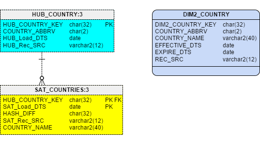
Figure 2 – Projecting a Type 2 Dimension from a Raw Vault

Type 1 Dimension for an Information Mart

This is very similar in structure and code as the Type 1 for the Raw Mart. The only difference is that the Dimension is built using tables that may be in the Raw Vault and in the Business Vault. For the example, I will show you a dimension for Employee data. To build a comprehensive Employee dimension, I need to include the Point-in-Time (PIT) table that we built in the prior article on Business Vault.

The SQL to project the Type 1 dimension, using the PIT table for Employees is this:

  SELECT
    PIT.HUB_EMPLOYEE_KEY AS DIM1_EMPLOYEE_KEY,
    PIT.PIT_LOAD_DTS     AS EFFECTIVE_DATE,
    HE.EMPLOYEE_ID,
    NM.FIRST_NAME,
    NM.LAST_NAME,
    NM.GENDER,
    NM.MARITAL_STATUS,
    NM.SSN,
    ADDR.ADDRESS1,
    ADDR.ADDRESS2,
    ADDR.CITY,
    ADDR.STATE,
    ADDR.POSTAL_CODE,
    ADDR.COUNTRY,
    CNTC.EMAIL,
    CNTC.PHONE_NUMBER,
    COMP.SALARY_BEGIN_DATE,
    COMP.SALARY,
    COMP.COMMISSION_PCT,
    SAL.MIN_SALARY,
    SAL.MAX_SALARY,
    SAL.AVG_SALARY,
    SAL.TOTAL_SALARY_TODATE
  FROM
    HUB_EMPLOYEE HE,
    EMPLOYEE_PIT PIT,
    SAT_EMPLOYEE_ADDRESS ADDR,
    SAT_EMPLOYEE_NAME NM,
    SAT_EMPLOYEE_CONTACTS CNTC,
    SAT_EMPLOYEE_COMPENSATION COMP,
    SAT_EMPLOYEE_SAL_SUM SAL
  WHERE HE.HUB_EMPLOYEE_KEY     = PIT.HUB_EMPLOYEE_KEY
  AND HE.HUB_EMPLOYEE_KEY       = ADDR.HUB_EMPLOYEE_KEY
  AND HE.HUB_EMPLOYEE_KEY       = NM.HUB_EMPLOYEE_KEY
  AND HE.HUB_EMPLOYEE_KEY       = CNTC.HUB_EMPLOYEE_KEY
  AND HE.HUB_EMPLOYEE_KEY       = COMP.HUB_EMPLOYEE_KEY
  AND HE.HUB_EMPLOYEE_KEY       = SAL.HUB_EMPLOYEE_KEY
  AND PIT.SAL_SUM_LOAD_DTS      = SAL.SAT_LOAD_DTS
  AND PIT.NAME_LOAD_DTS         = NM.SAT_Load_DTS
  AND PIT.ADDRESS_LOAD_DTS      = ADDR.SAT_Load_DTS
  AND PIT.CONTACT_LOAD_DTS      = CNTC.SAT_Load_DTS
  AND PIT.COMPENSATION_LOAD_DTS = COMP.SAT_Load_DTS
  AND PIT.PIT_LOAD_DTS         =
    (
      SELECT
        MAX(PIT2.PIT_LOAD_DTS)
      FROM
        EMPLOYEE_PIT PIT2
      WHERE
        HE.HUB_EMPLOYEE_KEY = PIT2.HUB_EMPLOYEE_KEY
    )

Just like the Type 1 for Raw Vault, this one also needs a MAX(Load Date) subquery to get the most current view of the data but in this case that is done against the PIT table. Without the PIT table, you would need these subqueries for every Satellite Load Date. (Remember this is one reason we suggest building a PIT table.)

Figure 3 shows the side-by-side model of the Data Vault tables and the resulting dimension.

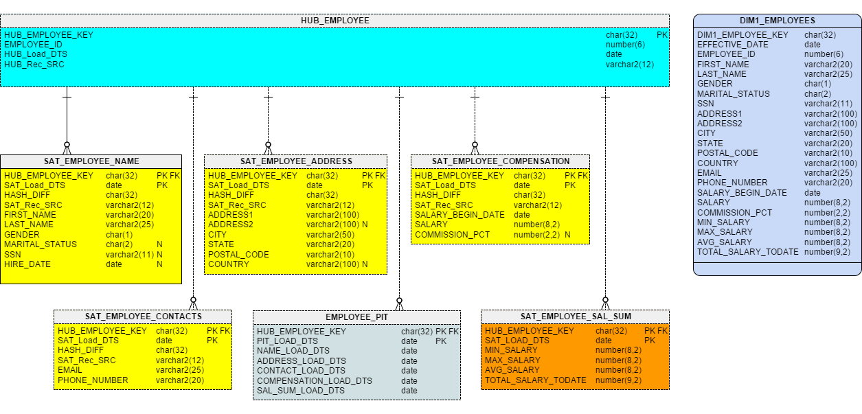
Figure 3 – Projecting a Type 1 Dimension from Business Vault

This picture makes it pretty clear why we generally do not let typical users query the Data Vault directly. The Dimension is much easier to understand.

Type 2 Dimension for an Information Mart

Just as we did against the Raw Vault, the Type 2 Dimension on a Business Vault needs a primary key (PK), and effective date and an expire date. The difference from the Raw Vault (in this case) is that the PK will be calculated using the Load Date from the PIT table rather than a standard Satellite table. And the Effective and Expire dates are also based on the PIT table.

SELECT
  dbms_obfuscation_toolkit.md5(upper(trim(HE.EMPLOYEE_ID))
  || '^'
  || TO_CHAR(PIT.PIT_LOAD_DTS, 'YYYY-MM-DD')) AS DIM2_EMPLOYEE_KEY,
  HE.EMPLOYEE_ID,
  PIT.PIT_LOAD_DTS AS EFFECTIVE_DATE,
  LEAD(PIT.PIT_LOAD_DTS) 
       OVER (PARTITION BY SC.HUB_EMPLOYEE_KEY 
             ORDER BY PIT.PIT_LOAD_DTS) EXPIRE_DTS,
  NM.FIRST_NAME,
  NM.LAST_NAME,
  NM.GENDER,
  NM.MARITAL_STATUS,
  NM.SSN,
  ADDR.ADDRESS1,
  ADDR.ADDRESS2,
  ADDR.CITY,
  ADDR.STATE,
  ADDR.POSTAL_CODE,
  ADDR.COUNTRY,
  CNTC.EMAIL,
  CNTC.PHONE_NUMBER,
  COMP.SALARY_BEGIN_DATE,
  COMP.SALARY,
  COMP.COMMISSION_PCT,
  SAL.MIN_SALARY,
  SAL.MAX_SALARY,
  SAL.AVG_SALARY,
  SAL.TOTAL_SALARY_TODATE
FROM
  HUB_EMPLOYEE HE,
  EMPLOYEE_PIT PIT,
  SAT_EMPLOYEE_ADDRESS ADDR,
  SAT_EMPLOYEE_NAME NM,
  SAT_EMPLOYEE_CONTACTS CNTC,
  SAT_EMPLOYEE_COMPENSATION COMP,
  SAT_EMPLOYEE_SAL_SUM SAL
WHERE HE.HUB_EMPLOYEE_KEY     = PIT.HUB_EMPLOYEE_KEY
AND HE.HUB_EMPLOYEE_KEY       = ADDR.HUB_EMPLOYEE_KEY
AND HE.HUB_EMPLOYEE_KEY       = NM.HUB_EMPLOYEE_KEY
AND HE.HUB_EMPLOYEE_KEY       = CNTC.HUB_EMPLOYEE_KEY
AND HE.HUB_EMPLOYEE_KEY       = COMP.HUB_EMPLOYEE_KEY
AND HE.HUB_EMPLOYEE_KEY       = SAL.HUB_EMPLOYEE_KEY
AND PIT.SAL_SUM_LOAD_DTS      = SAL.SAT_LOAD_DTS
AND PIT.NAME_LOAD_DTS         = NM.SAT_Load_DTS
AND PIT.ADDRESS_LOAD_DTS      = ADDR.SAT_Load_DTS
AND PIT.CONTACT_LOAD_DTS      = CNTC.SAT_Load_DTS
AND PIT.COMPENSATION_LOAD_DTS = COMP.SAT_Load_DTS

Without the PIT table, loading this dimension would be much more complicated as you would have to add all the Sat Load Dates to the PK calculation as well as align all the dates at points in time over history (as we discussed in the last article).

The resulting model for this is shown in Figure 4.

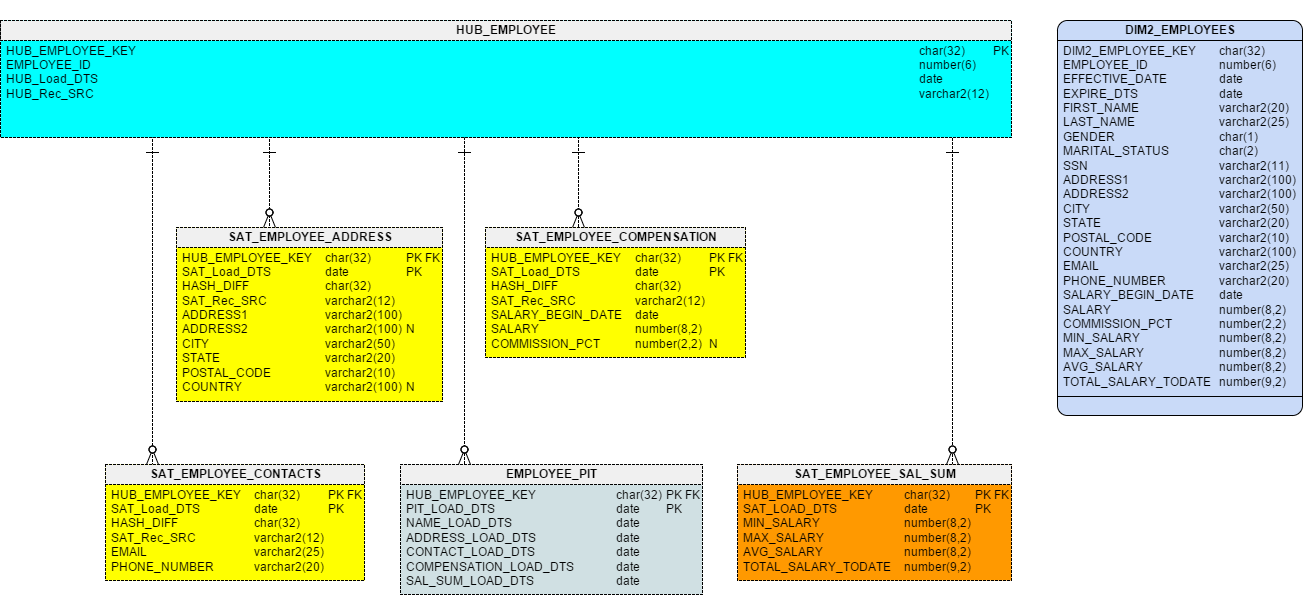
Figure 4 – Projecting a Type 2 Dimension from Business Vault

Fact Tables

In the Data Vault architecture, Fact tables are usually projected or derived from Link tables. In Data Vault, Link tables are where we load transactions. If you think about it, a Link is the intersection of two or more Hubs; a Fact is the intersection of two or more Dimensions. While it is true that there will be times when attributes in a Hub or Hub Satellite may contribute to a Fact table, in general this is not the case.

Just like with Dimensions, there are of course Fact tables projected into a Raw Data Mart from Raw Vault tables and then there are Fact tables projected into an Information Mart based on tables in the Business Vault.

Note that if you do not yet have any BV tables but do transformation as you build out the fact tables, you are in that case building an Information Mart structure rather than a Raw Data Mart (because you are applying business rules to the raw data).

Fact Table for a Raw Data Mart

Building a raw Fact table, with ties to Type 1 Dimensions is very straight forward. All the Hub Keys in the Link can become the Type 1 Dimension Keys for the Fact (if you define your dimensions like I showed above). The measures (or metrics) for the Fact will usually come from numeric attributes in the Link Satellite. Since the measure comes from the Satellite, then the record source and load date also need to come from the Sat as well in order to have a complete audit trail for that data.

Because Satellites contain changes over time, just like with Dimensions, we will need to filter for the most recent load date for a given Link record.

The SQL to create a Fact from one of the HR Link tables is show below:

SELECT
    LMD.HUB_EMPLOYEE_KEY   AS DIM1_EMPLOYEE_MANAGER_KEY,
    LMD.HUB_DEPARTMENT_KEY AS DIM1_DEPARTMENT_KEY,
    LMD.HUB_LOCATION_KEY   AS DIM1_LOCATION_KEY,
    SMD.ANNUAL_BUDGET,
    SMD.SAT_Load_DTS AS FACT_LOAD_DTS,
    SMD.SAT_Rec_SRC  AS FACT_REC_SRC
  FROM
    LNK_MANAGER_DEPARTMENTS LMD,
    SAT_MANAGER_DEPARTMENTS SMD
  WHERE
    LMD.LNK_DEPARTMENTS_KEY = SMD.LNK_DEPARTMENTS_KEY
  AND SMD.SAT_Load_DTS      =
    (
      SELECT
        MAX(SMD2.SAT_Load_DTS)
      FROM
        SAT_MANAGER_DEPARTMENTS SMD2
      WHERE
        LMD.LNK_DEPARTMENTS_KEY = SMD2.LNK_DEPARTMENTS_KEY
    )

Figure 5 displays the side-by-side model of the Link table and the Fact table.

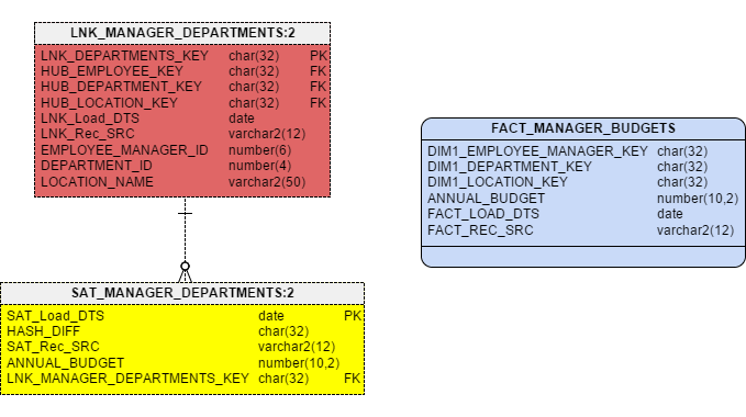
Figure 5 – Projecting a Fact from a Raw Vault

Note that the measure, ANNUAL_BUDGET, comes from the Satellite associated with the Link.

With this Fact table, users can now easily report on the current Annual Budget by Manager, Department, and Location. With the right BI tool, or a simple pivot table, users can also easily get summary and average budget numbers by Manager and Department, by Manager and Location, total budget for a Department, or total budget for a Location, along with several other combinations.

In terms of Agile BI, this one Fact table can be built and delivered very quickly to get the business users looking at their raw data. And if there are questions about the quality of the data, the Fact table includes the source of the data and when it was loaded to allow a complete data quality feedback loop for checking and auditing.

Because we applied no soft business rules in the transformation, technically this would be labeled as part of a Raw Data Mart, but as you might conclude, this data still provides a lot of value, very quickly, to the business users and so may be a candidate to put in the final Information Mart.

Fact Table for an Information Mart

By definition, Information Marts may have soft business rules or other transformations applied, so it follows that Fact tables built off the Business Vault would be candidates for inclusion. For the example, let’s look at the Bridge table we built in the last article. You may remember that a Bridge table is really a specialized Link that brings together the Keys from multiple Hubs and Links. Since it is a Link table, it is in fact a candidate to be transformed into a Fact table.

  SELECT
    BG.HUB_REGION_KEY   AS DIM1_REGION_KEY,
    BG.HUB_COUNTRY_KEY  AS DIM1_COUNTRY_KEY,
    BG.HUB_LOCATION_KEY AS DIM1_LOCATION_KEY,
    1                   AS GEO_COUNT,
    BG.BRDG_LOAD_DTS    AS FACT_LOAD_DTS
  FROM
    BRIDGE_GEOGRAPHY BG 

Figure 6 shows the result.

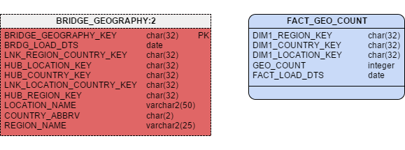
Figure 6 – Projecting a Fact from a Business Vault

Just as in the previous example, assuming we are using Type 1 Dimensions, the Dimension Keys for the Fact table are the Hub Keys found in the Bridge table. Since this bridge table has no pre-calculated numeric columns, I have also included a “counter” column to make aggregate reporting easier. In this case, the Bridge table really is the perfect basis for building what is often called a Fact-less Fact.

In Data Vault, nearly every Link table can be used to quickly build Fact-less Fact tables.

With this Fact table we can quickly check the number of Locations in a Country or the number of Countries in a Region. Assuming you have the appropriate Dimensions also in your Information Mart, you of course can filter the analysis by any of the attributes in those Dimensions.

Hopefully by now, you are seeing a pattern to all these SQL statements. Whether you are building a Type 1 or 2 Dimension or a Fact table, the basic logic is the same: start by joining Hub/Link + Sat then go from there.

This is because Data Vault is pattern-based and the load and extract logic rely on basic SQL and set theory.

Fact Tables with Type 2 Dimensions

Projecting Fact tables that use Type 2 Dimensions is hard regardless of your architecture. You have to first build your Type 2 Dimensions, with the “surrogate” PKs, then you can populate the Fact table by looking up the Dimensions Keys based on Business Keys and the date of the Fact record and the effective date of the Dimension records.

You would need to follow the same process with Data Vault. One advantage with Data Vault 2.0 in this instance is that the Link tables have the Business Keys already denormalized into the structure (see Figures 5 and 6). So, when you look to find the Type 2 Dimension Key, you will not need to do an additional lookup from the Link table to the Hub to find the matching Business Key. This should substantially improve the performance of that load process.

Final Data model

Virtualizing Your Marts

A recent trend in the data warehouse world has been about creating virtual data warehouses and data marts. With Data Vault 1.0 and 2.0, using what I have shown you in this article, it is very reasonable for you to create virtual marts.

All of the SQL code you have seen can be turned into views in the database. All you need to do is add CREATE VIEW as to the front of the SQL in this article.

I have done this successfully in both Oracle and SQL Server already and know others who have done so as well.

So why should you consider using views to build your Information Marts?

1. It supports an Agile project approach
   • Shorter iterations
   • Faster time to market
2. It eliminates ETL development bottlenecks
   • No need to write specs
   • No ETL programming or coding
   • Greatly reduces the amount and complexity of testing

By minimizing the amount of ETL coding needed upfront, you can greatly increase the speed at which you can deliver data to your customers.

I call that a win-win!

What about Performance?

Fair question.

It depends on many factors such as your RDBMS, your hardware (Exadata?), number of CPUs, and memory. But you should not assume it will be too slow. There have been so many advances in the last few years that we need to test the old assumptions!

Start by using the views and show the data. Then if it is too slow for production, you can always tune your database (maybe partition the base tables?), convert to Materialized Views or just build out the tables the old-fashioned way.

The key here is you do that in another iteration of the project, not the first time through. In agile terms, that is often called refactoring – and it is expected over time.

Series Conclusion

Well, that is the end of my series on Data Vault 2.0 Modeling and Methodology. In it I gave you some of the history about Data Vault and why you might consider using it for your Enterprise Data Warehouse architecture. I took you through the basics of modeling a Raw Data Vault with Hub, Links, and Satellites. Then we looked at the concept of a Business Vault and some typical constructs used there. Finally in this article we come to the end of the data trail with how to build a dimensional reporting layer for your end users.

I hope this has been an educational series for you and that you will know go forward to use Data Vault 2.0 in your work.

Want more in-depth details? Check out the online training available through http://LearnDataVault.com. As a special for Vertabelo readers, you can use the coupon code VERTABELO20 to get 20% off any online class from now until June 30, 2016. Don’t let the chance go by to learn more about Data Vault.

And don’t forget to order the new Data Vault 2.0 book on Amazon.com.

If you want some one-on-one coaching or formal Data Vault 2.0 training, please feel free to contact my via my blog. And please follow me on twitter @kentgraziano.

Carry on my friends.

Kent Graziano, CDVM2

The Data Warrior